Prepare AutoSort#
In this tutorial, we demonstrate how to train a AutoSort model with early-stage recordings and validate its performance.
For explanatory data analysis, we provide two days’ recording on 0310 and 0315, which can be downloaded here.
[1]:
from autosort_neuron import *
import warnings
warnings.filterwarnings("ignore")
/n/holystore01/LABS/jialiu_lab/Users/yichunhe/AutoSort/autosort_neuron/sorting.py:19: DeprecationWarning: The 'toolkit' module is deprecated. Use spikeinterface.preprocessing/postptocessing/qualitymetrics instead
  import spikeinterface.toolkit as st
[<torch.cuda.device object at 0x151035c7b880>]
Perform spike sorting with MountainSort and manual curation to get reference units#
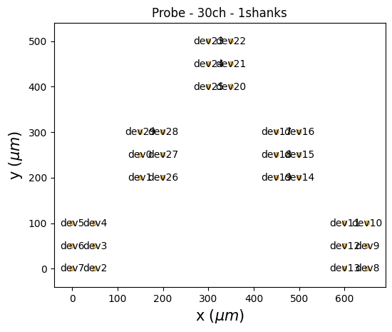
First, we need to define the geometry of the high-density probe
[2]:
positions=np.array([
                [150, 250], ### electrode 1 x,y
                [150,200], ### electrode 2 x,y
                [50, 0], ### electrode 3 x,y
                [50, 50],
                [50, 100],
                [0, 100],
                [0, 50],
                [0, 0],
                [650, 0],
                [650, 50],
                [650, 100],
                [600, 100],
                [600, 50],
                [600, 0],
                [500, 200],
                [500, 250],
                [500, 300],
                [450, 300],
                [450, 250],
                [450, 200],
                [350, 400],
                [350, 450],
                [350, 500],
                [300, 500],
                [300, 450],
                [300, 400],
                [200, 200],
                [200, 250],
                [200, 300],
                [150, 300]
                    ])
[3]:
mesh_probe = create_mesh_probe(positions=positions,num_all_channels=positions.shape[0])
plot_probe(mesh_probe,with_device_index=True)
[3]:
(<matplotlib.collections.PolyCollection at 0x15103495f5b0>, None)
Next, we load raw data recorded through Intan system. We read two days’ recording on 0310 and 0315, concatenate them.
[4]:
### raw data path
raw_data_path = './raw_data/'

### file folder name to read
date_id_all=['0310','0315']
save_folder_name = '_'.join(date_id_all)

### processed data path
data_folder_all = f'./processed_data/Ephys_concat_{save_folder_name}/'


sorting_method="mountainsort"
sorting_save_path = data_folder_all + sorting_method + '/'
[5]:
recording_concat, day_length = read_data_folder(data_folder_all,
                                                date_id_all,
                                                raw_data_path,
                                                mesh_probe, )

### bandpass filter and common reference

freq_max=3000
freq_min=300

recording_f = spikeinterface.preprocessing.bandpass_filter(recording_concat, freq_min=freq_min,
                                                   freq_max=freq_max)
recording_cmr = spikeinterface.preprocessing.common_reference(recording_f, reference='global',operator='average')
loading from existing folder: ./processed_data/Ephys_concat_0310_0315/
BinaryFolderRecording: 30 channels - 1 segments - 10.0kHz - 2046.387s
Num. channels = 30
Sampling frequency = 10000 Hz
Num. timepoints seg0= 1
We perform MountainSort spike sorting on the concatenated data.
[6]:
if os.path.exists(sorting_save_path)==False:
    os.mkdir(sorting_save_path)
output_folder = sorting_save_path + '/sorting'
firing_save_path = output_folder + f'/firings.npz'
[7]:
default_params = {
        'detect_sign': -1,  # Use -1, 0, or 1, depending on the sign of the spikes in the recording
        'adjacency_radius': 120,  # Use -1 to include all channels in every neighborhood
        'freq_min': 300,  # Use None for no bandpass filtering
        'freq_max': 3000,
        'filter': True,
        'whiten': True,  # Whether to do channel whitening as part of preprocessing
        'num_workers': 9,
        'clip_size': 50,
        'detect_threshold': 4, # 5
        'detect_interval': 3,  # Minimum number of timepoints between events detected on the same channel, 30
    }

fs = 10000
[8]:
if not os.path.exists(firing_save_path):
    sorting_wave_clus = ss.run_sorter(sorter_name='mountainsort4',
                                     recording=recording_cmr,
                                     remove_existing_folder='True',
                                     output_folder=output_folder,
                                     **default_params,)


    keep_unit_ids = []
    for unit_id in sorting_wave_clus.unit_ids:
        spike_train = sorting_wave_clus.get_unit_spike_train(unit_id=unit_id)
        n = spike_train.size
        if(n>20):
            keep_unit_ids.append(unit_id)

    curated_sorting = sorting_wave_clus.select_units(unit_ids=keep_unit_ids, renamed_unit_ids=None)
    NpzSortingExtractor.write_sorting(curated_sorting, firing_save_path)

sorting = se.NpzSortingExtractor(firing_save_path)
After spike sorting with MountainSort, we extract waveforms to manually curate units.
[9]:
pack_folder = sorting_save_path
waveform_folder = pack_folder + 'waveforms'
# shutil.rmtree(waveform_folder)
we = spikeinterface.extract_waveforms(recording_cmr, sorting, waveform_folder,
    load_if_exists=True,
    ms_before=1, ms_after=2., max_spikes_per_unit=1000000,
    chunk_size=30000)
[10]:
we.recording.set_probe(mesh_probe, in_place=True)
sorting_day_split(sorting, date_id_all, day_length, pack_folder,
                  sorting_save_name='firings_inlier')

<Figure size 640x480 with 0 Axes>
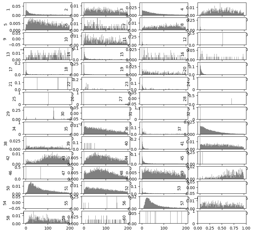
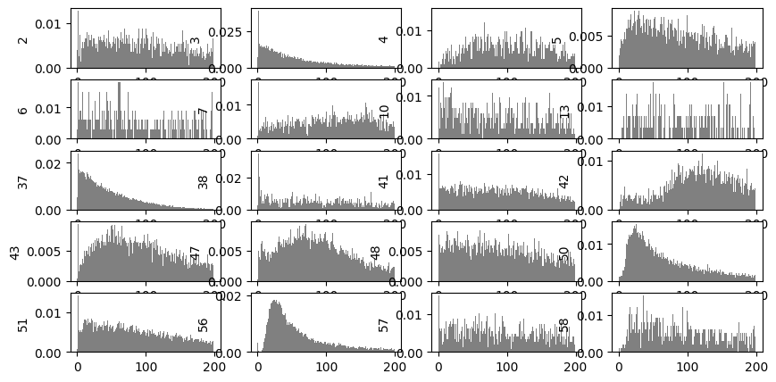
[11]:
fig,ax = plt.subplots(int(ceil(sorting.unit_ids.shape[0]/4)),4,figsize=(10,10))
sw.plot_isi_distribution(sorting, window_ms=200.0, bin_ms=1.0,axes=ax)
[11]:
<spikeinterface.widgets._legacy_mpl_widgets.isidistribution.ISIDistributionWidget at 0x151034504940>
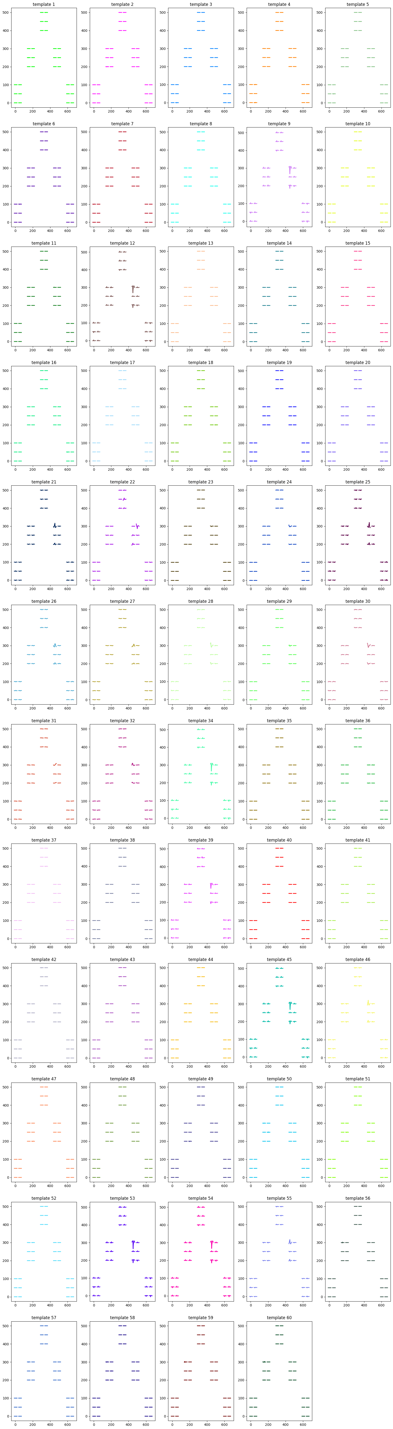
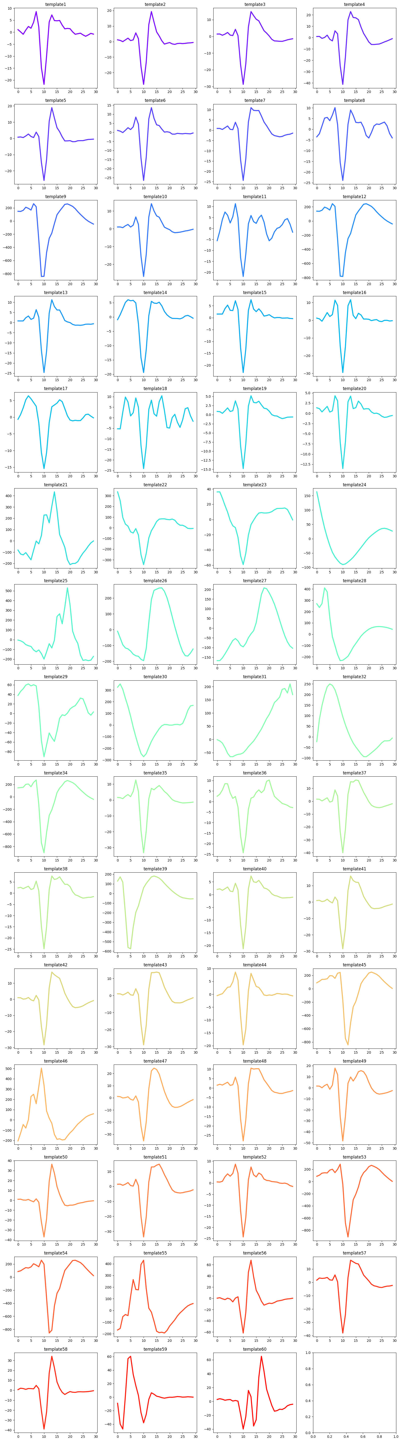
[12]:
# we._template_cache={}
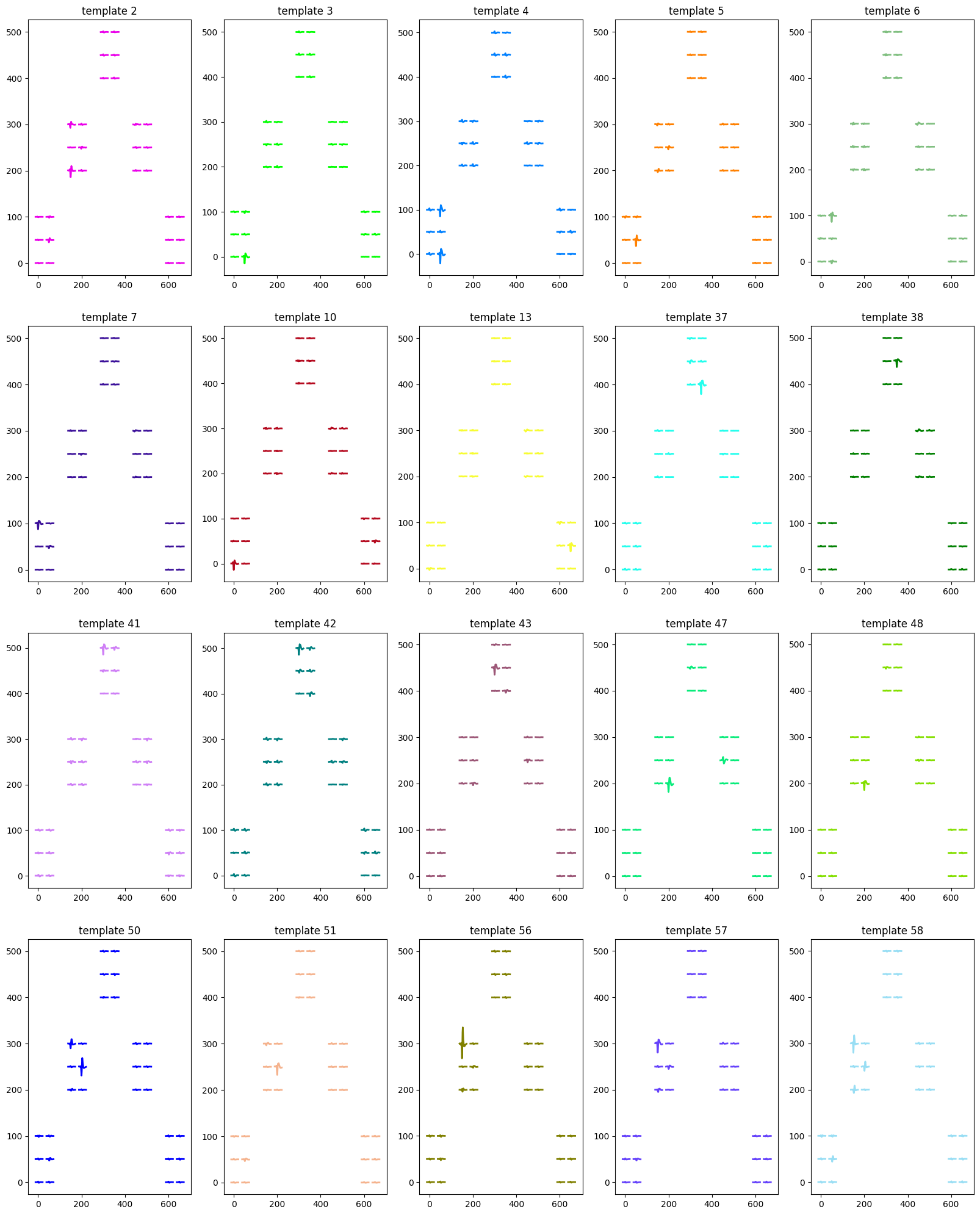
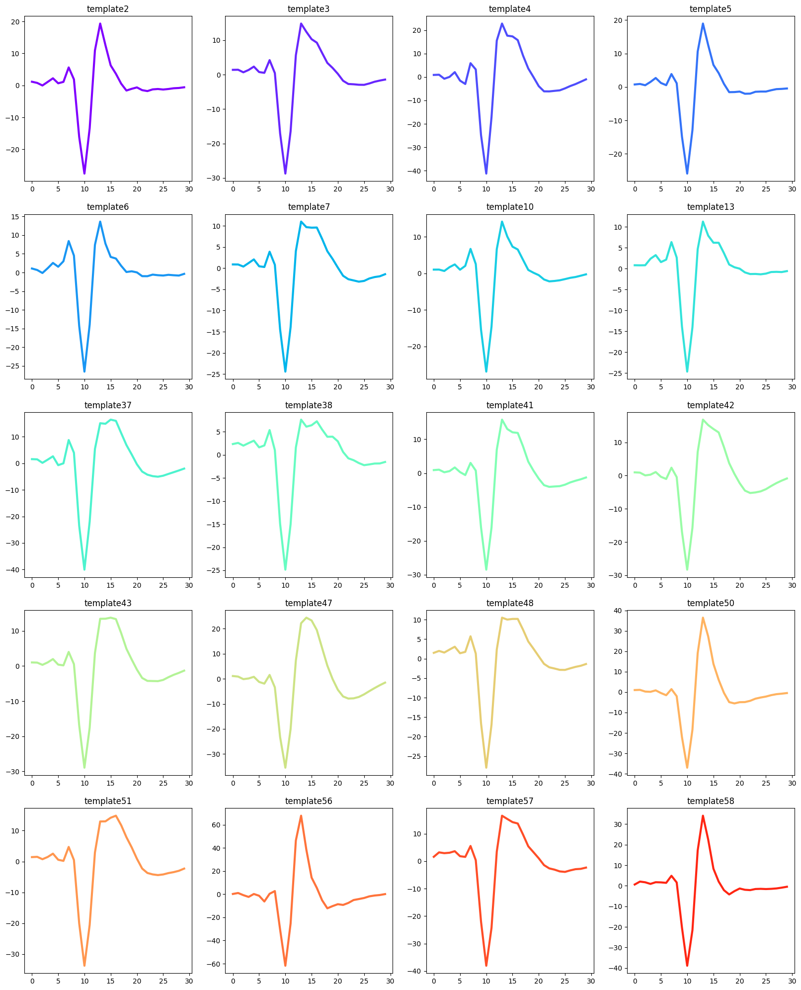
sorting_unit_show(we, recording_cmr, sorting, pack_folder,waveform_folder)
Through ISI, waveform characteristics and spiking patterns, we keep units ID 2,3,4,5,6,7,10,13,37,38,41,42,43,47,48,50,51,56,57,58.
[13]:
x=list(np.arange(1,np.max(sorting.unit_ids)+1))
y=[2,3,4,5,6,7,10,13,37,38,41,42,43,47,48,50,51,56,57,58]
left = [item for item in x if item not in y]

merge_unit_ids_pack = []
delete_unit_ids_pack = left
we_load_if_exists = True
waveform_show = False
input_state = 'merged'

curation_save_folder = pack_folder + f'/curation_result_{input_state}/'
if os.path.exists(curation_save_folder)==False:
    os.mkdir(curation_save_folder)

sorting,we = units_merge(recording_cmr, sorting, merge_unit_ids_pack, delete_unit_ids_pack,pack_folder, True)
[14]:
sorting_day_split(sorting, date_id_all, day_length, pack_folder,
                  sorting_save_name='firings_merged')

<Figure size 640x480 with 0 Axes>
We extract waveforms and the extremum channel of curated units.
[15]:
we._template_cache=[]
we.run_extract_waveforms()

probe_groups = np.arange(0,30)
NUmShanks = 30
we_load_if_exists = True

extremum_channels_ids = st.get_template_extremum_channel(we, peak_sign='neg')

pd.DataFrame.from_dict(extremum_channels_ids, orient='index').to_csv(pack_folder+'extremum_channels_ids.csv')
Plot waveforms and ISI of curated units.
[16]:
we._template_cache={}
sorting_unit_show(we, recording_cmr, sorting, pack_folder,waveform_folder)
[17]:
fig,ax = plt.subplots(int(ceil(sorting.unit_ids.shape[0]/4)),4,figsize=(10,5))
sw.plot_isi_distribution(sorting, window_ms=200.0, bin_ms=1.0,axes=ax)
[17]:
<spikeinterface.widgets._legacy_mpl_widgets.isidistribution.ISIDistributionWidget at 0x150dbaf8bee0>
Now, we can reformat information of sorted spikes as input for AutoSort
[18]:
save_pth = './AutoSort_data/'
day_pth = './processed_data/'
raw_data_path = './raw_data/'

freq_max=3000
freq_min=300

left_sample=10
right_sample=20
[ ]:
generate_autosort_input(date_id_all,
                            raw_data_path,
                            save_pth,
                            day_pth,
                            left_sample,
                            right_sample,
                            freq_min,
                            freq_max,
                            mesh_probe
                            )
processing: 0310
-- loading from existing folder: ./processed_data/Ephys_0310/
saving to: ./processed_data/Ephys_concat_0310/
write_binary_recording with n_jobs = 1 and chunk_size = None
BinaryFolderRecording: 30 channels - 1 segments - 10.0kHz - 1800.000s
Num. channels = 30
Sampling frequency = 10000 Hz
Num. timepoints seg0= 1
processing: 0315
-- loading from existing folder: ./processed_data/Ephys_0315/
saving to: ./processed_data/Ephys_concat_0315/
write_binary_recording with n_jobs = 1 and chunk_size = None
BinaryFolderRecording: 30 channels - 1 segments - 10.0kHz - 246.387s
Num. channels = 30
Sampling frequency = 10000 Hz
Num. timepoints seg0= 1
### 0310
### 1. load raw data
### 2. detect spikes
### 3. load ground truth
100%|██████████| 20/20 [00:00<00:00, 1225.60it/s]
### 4. map ground truth annotation
---spike detection rate: 0.9905178317441922
### 4.5 add all gt
### 5. find corresponding waveform
87%|████████▋ | 26/30 [03:50<02:00, 30.18s/it]
The input to AutoSort is under the folder ‘./AutoSort_data/’
Train a AutoSort model.#
[21]:
### group ID of each electrode 1,2,3...
electrode_group=[1, 1, 0, 0, 0, 0, 0, 0, 4, 4, 4, 4, 4, 4, 3, 3, 3, 3, 3, 3, 2, 2, 2, 2, 2, 2, 1, 1, 1, 1]
electrode_position=np.hstack([positions,np.array(electrode_group).reshape(-1,1)])
Set parameters of AutoSort
[22]:
args=config()
args.day_id_str=date_id_all ### all days
args.cluster_path='./AutoSort_data/' ### path of input data
args.set_time=0  ### set 0310 data as training data
args.test_time=[1] ### set 0315 data as testing data
args.group=np.arange(30)  ### all electrodes
args.samplepoints=left_sample+right_sample ### 30 points for each waveform
args.sensor_positions_all=electrode_position
[23]:
run(args)
---------------------------------- SEED ALL ----------------------------------
                           Seed Num :   0
---------------------------------- SEED ALL ----------------------------------
<autosort_neuron.config.config object at 0x1519e0f36370>
pred_location (139245, 3)
epoch : 1/20
100%|██████████| 218/218 [00:09<00:00, 23.59it/s]
epoch : 1/20, loss 1 = 0.000000, loss 2 = 330.640511,, loss 3 = 740.988600
100%|██████████| 55/55 [00:00<00:00, 66.18it/s]
epoch : 1/20, val loss 1 = 0.000000, loss 2 = 4.114871,loss 3 = 9.640091
Validation Loss Decreased(inf--->13.754963)   Saving The Model
epoch : 2/20
100%|██████████| 218/218 [00:03<00:00, 58.81it/s]
epoch : 2/20, loss 1 = 0.000000, loss 2 = 193.178763,, loss 3 = 423.306925
100%|██████████| 55/55 [00:00<00:00, 85.66it/s]
epoch : 2/20, val loss 1 = 0.000000, loss 2 = 2.847722,loss 3 = 6.419589
Validation Loss Decreased(13.754963--->9.267310)      Saving The Model
epoch : 3/20
100%|██████████| 218/218 [00:03<00:00, 58.07it/s]
epoch : 3/20, loss 1 = 0.000000, loss 2 = 143.481579,, loss 3 = 278.339883
100%|██████████| 55/55 [00:00<00:00, 80.82it/s]
epoch : 3/20, val loss 1 = 0.000000, loss 2 = 2.507965,loss 3 = 4.465588
Validation Loss Decreased(9.267310--->6.973553)       Saving The Model
epoch : 4/20
100%|██████████| 218/218 [00:03<00:00, 57.30it/s]
epoch : 4/20, loss 1 = 0.000000, loss 2 = 111.616244,, loss 3 = 191.615472
100%|██████████| 55/55 [00:00<00:00, 84.30it/s]
epoch : 4/20, val loss 1 = 0.000000, loss 2 = 2.090885,loss 3 = 3.172255
Validation Loss Decreased(6.973553--->5.263139)       Saving The Model
epoch : 5/20
100%|██████████| 218/218 [00:03<00:00, 58.01it/s]
epoch : 5/20, loss 1 = 0.000000, loss 2 = 84.410176,, loss 3 = 135.986480
100%|██████████| 55/55 [00:00<00:00, 83.64it/s]
epoch : 5/20, val loss 1 = 0.000000, loss 2 = 2.073249,loss 3 = 2.364286
Validation Loss Decreased(5.263139--->4.437535)       Saving The Model
epoch : 6/20
100%|██████████| 218/218 [00:03<00:00, 58.10it/s]
epoch : 6/20, loss 1 = 0.000000, loss 2 = 64.752462,, loss 3 = 100.513181
100%|██████████| 55/55 [00:00<00:00, 84.60it/s]
epoch : 6/20, val loss 1 = 0.000000, loss 2 = 1.785286,loss 3 = 1.800739
Validation Loss Decreased(4.437535--->3.586025)       Saving The Model
epoch : 7/20
100%|██████████| 218/218 [00:03<00:00, 57.45it/s]
epoch : 7/20, loss 1 = 0.000000, loss 2 = 48.028065,, loss 3 = 75.402992
100%|██████████| 55/55 [00:00<00:00, 84.74it/s]
epoch : 7/20, val loss 1 = 0.000000, loss 2 = 2.365495,loss 3 = 1.395947
epoch : 8/20
100%|██████████| 218/218 [00:03<00:00, 58.42it/s]
epoch : 8/20, loss 1 = 0.000000, loss 2 = 36.942173,, loss 3 = 59.012671
100%|██████████| 55/55 [00:00<00:00, 84.06it/s]
epoch : 8/20, val loss 1 = 0.000000, loss 2 = 3.124771,loss 3 = 1.103077
epoch : 9/20
100%|██████████| 218/218 [00:03<00:00, 58.74it/s]
epoch : 9/20, loss 1 = 0.000000, loss 2 = 28.823177,, loss 3 = 46.371493
100%|██████████| 55/55 [00:00<00:00, 85.58it/s]
epoch : 9/20, val loss 1 = 0.000000, loss 2 = 2.048367,loss 3 = 0.906828
Validation Loss Decreased(3.586025--->2.955195)       Saving The Model
epoch : 10/20
100%|██████████| 218/218 [00:03<00:00, 57.09it/s]
epoch : 10/20, loss 1 = 0.000000, loss 2 = 22.871423,, loss 3 = 37.524615
100%|██████████| 55/55 [00:00<00:00, 85.60it/s]
epoch : 10/20, val loss 1 = 0.000000, loss 2 = 3.207553,loss 3 = 0.789877
epoch : 11/20
100%|██████████| 218/218 [00:03<00:00, 58.54it/s]
epoch : 11/20, loss 1 = 0.000000, loss 2 = 17.747776,, loss 3 = 31.112469
100%|██████████| 55/55 [00:00<00:00, 85.87it/s]
epoch : 11/20, val loss 1 = 0.000000, loss 2 = 3.440332,loss 3 = 0.664548
epoch : 12/20
100%|██████████| 218/218 [00:03<00:00, 58.06it/s]
epoch : 12/20, loss 1 = 0.000000, loss 2 = 15.388322,, loss 3 = 26.073921
100%|██████████| 55/55 [00:01<00:00, 45.63it/s]
epoch : 12/20, val loss 1 = 0.000000, loss 2 = 2.443036,loss 3 = 0.541770
epoch : 13/20
100%|██████████| 218/218 [00:06<00:00, 33.17it/s]
epoch : 13/20, loss 1 = 0.000000, loss 2 = 15.040105,, loss 3 = 20.390552
100%|██████████| 55/55 [00:00<00:00, 79.12it/s]
epoch : 13/20, val loss 1 = 0.000000, loss 2 = 2.879471,loss 3 = 0.528056
epoch : 14/20
100%|██████████| 218/218 [00:04<00:00, 45.45it/s]
epoch : 14/20, loss 1 = 0.000000, loss 2 = 14.558989,, loss 3 = 16.567875
100%|██████████| 55/55 [00:00<00:00, 82.36it/s]
epoch : 14/20, val loss 1 = 0.000000, loss 2 = 3.033507,loss 3 = 0.477917
epoch : 15/20
100%|██████████| 218/218 [00:03<00:00, 57.26it/s]
epoch : 15/20, loss 1 = 0.000000, loss 2 = 11.740852,, loss 3 = 15.012247
100%|██████████| 55/55 [00:00<00:00, 80.93it/s]
epoch : 15/20, val loss 1 = 0.000000, loss 2 = 3.372676,loss 3 = 0.360178
epoch : 16/20
100%|██████████| 218/218 [00:03<00:00, 57.89it/s]
epoch : 16/20, loss 1 = 0.000000, loss 2 = 11.570271,, loss 3 = 12.874262
100%|██████████| 55/55 [00:00<00:00, 85.54it/s]
epoch : 16/20, val loss 1 = 0.000000, loss 2 = 2.838299,loss 3 = 0.376539
epoch : 17/20
100%|██████████| 218/218 [00:09<00:00, 23.30it/s]
epoch : 17/20, loss 1 = 0.000000, loss 2 = 11.579632,, loss 3 = 10.456739
100%|██████████| 55/55 [00:02<00:00, 18.61it/s]
epoch : 17/20, val loss 1 = 0.000000, loss 2 = 4.333641,loss 3 = 0.337019
epoch : 18/20
100%|██████████| 218/218 [00:12<00:00, 18.14it/s]
epoch : 18/20, loss 1 = 0.000000, loss 2 = 9.196238,, loss 3 = 9.392744
100%|██████████| 55/55 [00:01<00:00, 52.27it/s]
epoch : 18/20, val loss 1 = 0.000000, loss 2 = 3.623895,loss 3 = 0.315759
epoch : 19/20
100%|██████████| 218/218 [00:09<00:00, 23.35it/s]
epoch : 19/20, loss 1 = 0.000000, loss 2 = 10.644902,, loss 3 = 8.946619
100%|██████████| 55/55 [00:01<00:00, 30.24it/s]
epoch : 19/20, val loss 1 = 0.000000, loss 2 = 1.640556,loss 3 = 0.290822
Validation Loss Decreased(2.955195--->1.931378)       Saving The Model
epoch : 20/20
100%|██████████| 218/218 [00:05<00:00, 36.85it/s]
epoch : 20/20, loss 1 = 0.000000, loss 2 = 13.910450,, loss 3 = 7.684290
100%|██████████| 55/55 [00:00<00:00, 84.45it/s]
epoch : 20/20, val loss 1 = 0.000000, loss 2 = 2.211047,loss 3 = 0.447237
pred_location (138641, 3)
100%|██████████| 271/271 [00:03<00:00, 81.89it/s]
The trained model is saved in ‘./AutoSort_data/model_save/train_day0305_0/train_weight’.
We will load it for spike sorting of later-stage recordings.
We read the training and testing log to check results.
[27]:
training_log=pd.read_csv('/n/holystore01/LABS/jialiu_lab/Users/yichunhe/AutoSort/AutoSort_data/model_save/train_day0310_0/train_weight/training_log.csv',
index_col=0)

test_log=pd.read_csv('/n/holystore01/LABS/jialiu_lab/Users/yichunhe/AutoSort/AutoSort_data/model_save/train_day0310_0/train_weight/test_log.csv',
index_col=0)
[28]:
training_log
[28]:
| epoch | validation_acc_noise | validation_acc_label | |
|---|---|---|---|
| 0 | 1 | 0.894969 | 0.933277 |
| 1 | 2 | 0.932134 | 0.966554 |
| 2 | 3 | 0.939280 | 0.972466 |
| 3 | 4 | 0.942619 | 0.977872 |
| 4 | 5 | 0.947036 | 0.976689 |
| 5 | 6 | 0.945097 | 0.979223 |
| 6 | 7 | 0.943625 | 0.980743 |
| 7 | 8 | 0.949837 | 0.984291 |
| 8 | 9 | 0.947574 | 0.982095 |
| 9 | 10 | 0.950124 | 0.983953 |
| 10 | 11 | 0.950806 | 0.983784 |
| 11 | 12 | 0.945815 | 0.984122 |
| 12 | 13 | 0.949801 | 0.982939 |
| 13 | 14 | 0.950339 | 0.983108 |
| 14 | 15 | 0.946677 | 0.982432 |
| 15 | 16 | 0.946856 | 0.983953 |
| 16 | 17 | 0.951057 | 0.984291 |
| 17 | 18 | 0.951345 | 0.982432 |
| 18 | 19 | 0.940536 | 0.984628 |
| 19 | 20 | 0.944558 | 0.983446 |
[29]:
test_log
[29]:
| train_time | timepoint | noise_acc | label_acc | |
|---|---|---|---|---|
| 0 | 305 | 310 | 0.985848 | 0.997155 |
[ ]: